There’s been a lot of work in the Haskell ecosystem that has made it easier to write interactive Kaggle-like scripts. I’d like to showcase the synergy between 3 such tools: dataframe (my own creation), hasktorch, and IHaskell.

At a high level the intent of this post is to:

• get people excited about how far the ecosystem has come,
• checkpoint what the ecosystem currently looks like,
• identify areas of improvement in the workflow.

This post is a narrative companion to a hosted notebook, but with a little more context.

This work was done as part of the dataHaskell: an organization devoted to enabling reliable and reproducible machine learning using the Haskell programming language.

Special thanks to Jireh Tan for writing the code.

The iris classification problem

The Iris dataset is machine learning’s “Hello, World!” created by statistician Ronald Fisher in 1936. The dataset contains measurements of 150 iris flowers from three species:

• Setosa
• Versicolor
• Virginica

For each flower, we have four measurements (in centimetres):

• Sepal length and width (the green outer part)
• Petal length and width (the colourful inner part)

Our task is to predict the species of a flower given these four measurements.

Loading and Exploring the Data

We start by loading the data from a Parquet file using the DataFrame library:

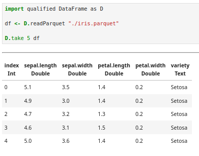
One immediate advantage of Haskell: the type system tells us we have no missing values. If any column contained nulls we’d see a Maybe prefix in front of that type. At least in this case, we don’t have to worry about deciding between imputing data and dropping it.

Exploring our data

Checking for balance

Before building any model, we need to know if our dataset is balanced. A severely imbalanced dataset (say, 140 Setosas and 5 each of the others) would make accurate prediction nearly impossible.

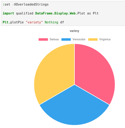
Great! A perfect balance with 50 flowers of each species. This means we don’t have to spend time on rebalancing tricks.

Some light analysis

Next, we compare feature magnitudes per class. We unintuitively do this in a stacked bar chart. But since our plot is interactive and allows us to exclude features at the click of a button we throw them all in there then click around to look at their individual differences.

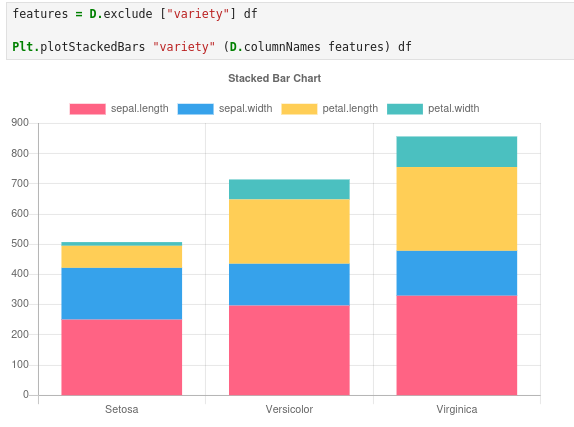
Our charts broadly suggest that Virginica > Versicolor > Setosa for most features, with one fun exception: Setosa has the largest sepal width.

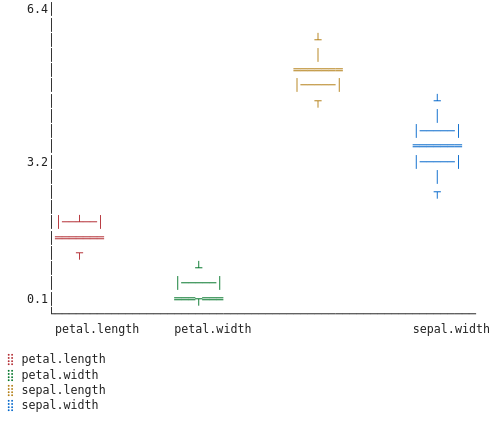
To get a sense of the spread of the features we can do box plots per variety and compare them:

Since we don’t have box plots implemented as web plots we fall back to granite’s ASCII plot.

For Setosa:

For Versicolor

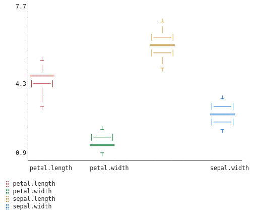
For Virginica:

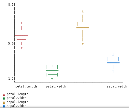
The box plots reveal that Setosas should be easy to identify—their petals are tiny with little variance. Versicolors and Virginicas overlap more, but we can still try to distinguish them using feature engineering.

Creating new features

From our exploration we have 5 promising feature candidates:

• sepal area
• sepal length to width ratio
• petal area
• petal length to width ratio
• sepal area / petal area

To derive these feature it’ll help to create typed references to the columns using template Haskell. This is the equivalent of doing a database migration against a schema definition. Except in this case we just freeze the types as they exist in the dataframe already.

:set -XTemplateHaskell
import qualified DataFrame.Functions as F

F.declareColumns df

import DataFrame ((|>))

engineered = df
               |> D.derive "sepal_area" (sepal_length * sepal_width)
               |> D.derive "sepal_ratio" (sepal_length / sepal_width)
               |> D.derive "petal_area" (petal_length * petal_width)
               |> D.derive "petal_ratio" (petal_length / petal_width)
               |> D.derive "area_ratio" ((sepal_length * sepal_width) / (petal_length * petal_width))

After repeating the previous diagramming (see the full notebook) we decide we can get by with three features:

• petal_area,
• sepal_area, and,
• area_ratio

Creating a custom data type for our label

Here’s where Haskell’s type system shines. Instead of treating species as magic integers, we define them explicitly:

data Iris
    = Setosa
    | Versicolor
    | Virginica
    deriving (Eq, Show, Read, Ord, Enum)

The deriving clause automatically generates useful functions:

• Eq: Allows us to compare Iris values for equality
• Show: Converts Iris to a String (e.g., “Setosa”)
• Read: Converts a String to Iris (e.g., “Setosa” → Setosa)
• Ord: Allows ordering/sorting
• Enum: Lets us convert to/from integers (Setosa=0, Versicolor=1, Virginica=2)

We convert our string labels to this type:

import qualified Data.Text as T

modellingDf = D.select ["petal_area", "sepal_area", "area_ratio", "variety"] engineered
withTypedLabel =
        modellingDf
            |> D.derive
                "variety"
                (F.lift (fromEnum . read @Iris . T.unpack) variety)

Preparing our data for ML

For our model to generalise, we split the data: 70% for training, 30% for testing. Our random split function takes a seed and probability p. It return a tuple where (p * 100) % of the vakues are in the first element and the rest are in the second.

The random seed (42) ensures reproducibility which is crucial for debugging.

import qualified DataFrame.Hasktorch as DHT
import qualified System.Random as SysRand
import Control.Exception (throw)

let (trainDf, testDf) = D.randomSplit (SysRand.mkStdGen 42) 0.7 withTypedLabel

let trainFeaturesTr =
        trainDf
            |> D.exclude ["variety"]
            |> DHT.toTensor
let testFeaturesTr =
        testDf
            |> D.exclude ["variety"]
            |> DHT.toTensor

let trainLabels = either throw id (D.columnAsIntVector "variety" trainDf)
let testLabels = either throw id (D.columnAsIntVector "variety" testDf)

Since we are predicting one of many classes, our target should be a one-hot vector:

• 0 (Setosa) → [1.0, 0.0, 0.0]
• 1 (Versicolor) → [0.0, 1.0, 0.0]
• 2 (Virginica) → [0.0, 0.0, 1.0]

import qualified Torch as HT

let trainLabelsTr = HT.toType HT.Float (HT.oneHot 3 (HT.asTensor trainLabels))
let testLabelsTr = HT.toType HT.Float (HT.oneHot 3 (HT.asTensor $ testLabels))

The function application can be read from right to left:

• Make the label into a tensor
• Create a one-hot vector with three entries.
• Then finally convert each int to a float.

That’s it. Our data is ready for machine learning. Now we can pass it to Torch and use it to train a small multi-layer perceptron.

Training the model

Neural Network Architecture

We define our Multi-Layer Perceptron (MLP) architecture in two parts.

First, a specification that describes the shape of our network. Second, the actual model with its layers. Each layer is a Linear transformation (like nn.Linear in PyTorch).

:set -XDeriveGeneric
import qualified Torch as HT

import GHC.Generics (Generic)

data MLPSpec = MLPSpec
    { inputFeatures :: Int   -- Number of input features (3 for our dataset)
    , hiddenFeatures :: Int  -- Number of neurons in hidden layer
    , outputFeatures :: Int  -- Number of output classes (3 species)
    }
    deriving (Show, Eq)

data MLP = MLP
    { l0 :: HT.Linear  -- Input → Hidden layer
    , l1 :: HT.Linear  -- Hidden → Output layer
    }
    deriving (Generic, Show)

Network Architecture Diagram:

Input Layer (3)  →  Hidden Layer (8)  →  Output Layer (3)
---------------     -----------------     ----------------
sepal_area          ReLU activation       Softmax
petal_area          (introduces           (produces
area_ratio          non-linearity)        probabilities)
                                          Setosa
                                          Versicolor
                                          Virginica

Making Our Model Trainable

We need to tell Hasktorch how to initialise our network with random weights. This is similar to defining __init__() in a PyTorch nn.Module:

:set -XRecordWildCards

instance HT.Parameterized MLP
instance HT.Randomizable MLPSpec MLP where
    sample MLPSpec{..} =
        MLP
            <$> HT.sample (HT.LinearSpec inputFeatures hiddenFeatures)
            <*> HT.sample (HT.LinearSpec hiddenFeatures outputFeatures)

The <$> and <*> operators are Haskell’s way of working with random initialisation. Think of this as: “Create an MLP by randomly sampling weights for both layers.”

Forward Pass

This function defines how data flows through the network. It’s equivalent to the forward() method in PyTorch. Read it from right to left (or bottom to top in the chain):

mlp :: MLP -> HT.Tensor -> HT.Tensor
mlp MLP{..} =
    HT.softmax (HT.Dim 1)       -- 4. Apply softmax (probabilities sum to 1)
        . HT.linear l1          -- 3. Apply second linear layer
        . HT.relu               -- 2. Apply ReLU activation
        . HT.linear l0          -- 1. Apply first linear layer

Read this right-to-left (or bottom-to-top). The . operator composes functions.

In Python/PyTorch, this would look like:

def forward(self, x):
    x = self.l0(x)
    x = F.relu(x)
    x = self.l1(x)
    x = F.softmax(x, dim=1)
    return x

The Haskell version is directly captures that we are composing a series of functions and using the output of one as the input to the other.

Training Loop

Training longer doesn’t always mean better. At some point, your model starts memorizing the training data instead of learning general patterns.

We detect this by watching the test set loss. As long as test loss keeps decreasing, the model is learning generalizable patterns. But if training loss keeps dropping while test loss starts climbing, we’re overfitting.

This is called early stopping, and it’s one of the simplest yet most effective regularisation techniques in machine learning.

The Training State

Our training loop needs to track more than just the current model. We maintain:

• Current model: Updated every iteration
• Best model: The weights that gave us the lowest test loss
• Best loss: What that test loss was
• Patience counter: How many checks since we last improved?

If we don’t improve for several consecutive checks (in our case 5 iterations), we give up and return the best model we found.

The loop structure might look unusual if you’re coming from PyTorch. Instead of a for loop with mutation, we use the very similar looking foldLoop which takes a number of iterations, an initial state and a function that evolves that state with each iteration. Each iteration receives the previous state and returns the new state. No hidden mutable variables, just explicit data flow.

This is eventually the sort of thing we should abstract behind a good machine learning library but for now it’s easy enough to implement.

import Control.Monad (when)

trainLoop ::
    Int ->                          -- Number of epochs
    (HT.Tensor, HT.Tensor) ->       -- Training features and labels
    (HT.Tensor, HT.Tensor) ->       -- Test features and labels
    MLP ->                          -- Initial model
    IO MLP                          -- Returns trained model
trainLoop n trainingData testData initialModel = do
    let initialState = makeInitialState initialModel
    (_, bestModel, _, _) <- HT.foldLoop initialState n (trainingStep trainingData testData)
    pure bestModel
  where
    -- Configuration constants
    patience = 5
    checkInterval = 500
    learningRate = 1e-2
    initialBestLoss = read @Float "Infinity"
    
    -- Create initial training state
    makeInitialState model = (model, model, initialBestLoss, 0)
    
    -- Main training step for each iteration
    trainingStep (features, labels) (testFeatures, testLabels) (model, bestModel, bestLoss, counter) i
        | shouldStopEarly counter = pure (model, bestModel, bestLoss, counter)
        | otherwise = do
            -- Train and evaluate
            (updatedModel, trainLoss) <- performTrainingStep model features labels
            testLoss <- computeTestLoss updatedModel testFeatures testLabels
            
            -- Log progress periodically
            when (shouldLogProgress i) $
                logTrainingProgress i trainLoss testLoss
            
            -- Update best model tracking
            let (newBest, newBestLoss, newCounter) = 
                    updateBestModelTracking updatedModel testLoss bestModel bestLoss counter
            
            pure (updatedModel, newBest, newBestLoss, newCounter)
    
    -- Early stopping condition
    shouldStopEarly counter = counter >= patience
    
    -- Logging condition
    shouldLogProgress i = i `mod` checkInterval == 0
    
    -- Perform one training iteration
    performTrainingStep model features labels = do
        let predictions = mlp model features
            loss = HT.binaryCrossEntropyLoss' labels predictions
        (updatedModel, _) <- HT.runStep model HT.GD loss learningRate
        pure (updatedModel, HT.asValue loss :: Float)
    
    -- Evaluate model on test set
    computeTestLoss model features labels =
        let predictions = mlp model features
            loss = HT.binaryCrossEntropyLoss' labels predictions
        in pure (HT.asValue loss :: Float)
    
    -- Print training progress
    logTrainingProgress iteration trainLoss testLoss =
        putStrLn $ "Iteration: " ++ show iteration
                ++ " | Training Set Loss: " ++ show trainLoss
                ++ " | Test Set Loss: " ++ show testLoss
    
    -- Update best model if test loss improved, otherwise increment patience counter
    updateBestModelTracking currentModel currentLoss bestModel bestLoss counter =
        if currentLoss < bestLoss
            then (currentModel, currentLoss, 0)  -- New best: reset counter
            else (bestModel, bestLoss, counter + 1)  -- No improvement: increment counter

Running the training loop

We bring everything together by running our training loop with a model intialized from our MLPSpec.

initialModel <- HT.sample $ MLPSpec 3 8 3

trainedModel <-
    trainLoop
        10000
        (trainFeaturesTr, trainLabelsTr)
        (testFeaturesTr, testLabelsTr)
        initialModel

putStrLn "Your model weights are given as follows: "
print trainedModel

Evaluating the model

The notebook creates some helps to evaluate to the model. We’ll skip these details since most of the code is vanilla Haskell.

And for our results. Training metrics:

------------------------------------------
index |  variety   | precision |  recall  
------|------------|-----------|----------
 Int  |    Iris    |   Float   |   Float  
------|------------|-----------|----------
0     | Setosa     | 1.0       | 1.0      
1     | Versicolor | 0.9677419 | 0.9375   
2     | Virginica  | 0.9459459 | 0.9722222

Test metrics:

------------------------------------------
index |  variety   | precision |  recall  
------|------------|-----------|----------
 Int  |    Iris    |   Float   |   Float  
------|------------|-----------|----------
0     | Setosa     | 1.0       | 1.0      
1     | Versicolor | 1.0       | 0.8888889
2     | Virginica  | 0.875     | 1.0

Conclusion

This post demonstrates building a complete multiclass classification system in Haskell from scratch. We tackle the classic Iris dataset. The journey covers data loading, exploratory analysis, feature engineering, typed data modelling, network architecture design, training with early stopping, and evaluation.

The tools for a robust data science journey are scattered in the Haskell ecosystem. The hope is that we can unify them and along the way create ergonomic and safe APIs for data science.

Wanna join in this work?

Come over to the dataHaskell Discord to help shape the future of data science and Haskell?

The downloaded ipynb for this post can be found here.